10. The Affine Transformation Matrix (a.k.a. P)
- About this page
- Texture mapping and affine transformations.
- “Many of the truths we cling to depend greatly upon our own point of view.”
- Finishing up
- Tonc’s affine functions
About this page
As you probably know, the GBA is capable of applying geometric transformations like rotating and/or scaling to sprites and backgrounds. To set them apart from the regular items, the transformable ones are generally referred to as Rot/Scale sprites and backgrounds. The transformations are described by four parameters, pa, pb, pc and pd. The locations and exact names differ for sprites and backgrounds but that doesn’t matter for now.
There are two ways of interpreting these numbers. The first is to think of each of them as individual offsets to the sprite and background data. This is how the reference documents like GBATEK and CowBite Spec describe them. The other way is to see them as the elements of a 2x2 matrix which I will refer to as P. This is how pretty much all tutorials describe them. These tutorials also give the following matrix for rotation and scaling:
Now, this is indeed a rotation and scale matrix. Unfortunately, it’s also the wrong one! Or at least, it probably does not do what you’d expect. For example, consider the case with a scaling of = 1.5, = 1.0 and a rotation of α= 45. You’d probably expect something like fig 10.2a, but what you’d actually get is fig 10.2b. The sprite has rotated, but in the wrong direction, it has shrunk rather than expanded and there’s an extra shear as well. Of course, you can always say that you meant for this to happen, but that’s probably not quite true.
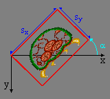
Fig 10.2a: when you say ‘rotate and scale’, you probably expect this…
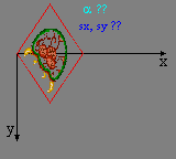
Fig 10.2b: but with P from eq 10.1, this is what you get.
Unfortunately, there is a lot of incorrect or misleading information on the transformation matrix around; the matrix of eq 10.1 is just one aspect of it. This actually starts with the moniker “Rot/Scale”, which does not fit with what actually occurs, continues with the fact that the terms used are never properly defined and that most people often just copy-paste from others without even considering checking whether the information is correct or not. The irony is that the principle reference document, GBATEK, gives the correct descriptions of each of the elements, but somehow it got lost in the translation to matrix form in the tutorials.
In this chapter, I’ll provide the correct interpretation of the P-matrix; how the GBA uses it and how to construct one yourself. To do this, though, I’m going into full math-mode. If you don’t know your way around vector and matrix calculations you may have some difficulties understanding the finer points of the text. There is an appendix on linear algebra for some pointers on this subject.
This is going to be a purely theoretical page: you will find nothing that relates directly to sprites or backgrounds here; that’s what the next two sections are for. Once again, we will be assisted by the lovely metroid (keep in cold storage for safe use). Please mind the direction of the y-axis and the angles, and do not leave without reading the finishing up paragraph. This contains several key implementation details that will be ignored in the text preceding it, because they will only get in the way at that point.
Be wary of documents covering affine parameters
It’s true. Pretty much every document I’ve seen that deals with this subject is problematic in some way. A lot of them give the wrong rotate-scale matrix (namely, the one in eq 10.1), or misname and/or misrepresent the matrix and its elements.
Texture mapping and affine transformations.
General 2D texture mapping
What the GBA does to get sprites and tiled backgrounds on screen is very much like texture mapping. So forget about the GBA right now and look at how texture mapping is done. In fig 10.4a, we see a metroid texture. For convenience I am using the standard Cartesian 2D coordinate system (y-axis points up) and have normalised the texture, which means that the right and top side of the texture correspond precisely with the unit-vectors and (which are of length 1). The texture mapping brings p (in texture space) to a point q (in screen space). The actual mapping is done by a 2×2 matrix A:
So how do you find A? Well, that’s actually not that hard. The matrix is formed by lining up the transformed base vectors, which are u and v (this works in any number of dimensions, btw), so that gives us:
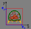
Fig 10.4a: a texture.
→
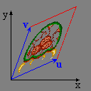
Fig 10.4b: a texture mapped
A forward texture mapping via affine matrix A.
Affine transformations
The transformations you can do with a 2D matrix are called affine transformations. The technical definition of an affine transformation is one that preserves parallel lines, which basically means that you can write them as matrix transformations, or that a rectangle will become a parallelogram under an affine transformation (see fig 10.4b).
Affine transformations include rotation and scaling, but also shearing. This is why I object to the name “Rot/Scale”: that term only refers to a special case, not the general transformation. It is akin to calling colors shades of red: yes, reds are colors too, but not all colors are reds, and to call them that would give a distorted view of the subject.
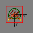
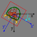
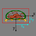
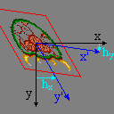
As I said, there are three basic 2d transformations, though you can always describe one of these in terms of the other two. The transformations are: rotation (R), scaling (S) and shear (H). Table 10.1 shows what each of the transformations does to the regular metroid sprite. The black axes are the normal base vectors (note that y points down!), the blue axes are the transformed base vectors and the cyan variables are the arguments of the transformation. Also given are the matrix and inverse matrix of each transformation. Why? You’ll see.
Table 10.1: transformation matrices and their inverses.
| Identity | Rotation | Scaling | Shear |
|---|---|---|---|
 |
 |
 |
 |
We can now use these definitions to find the correct matrix for enlargements by and , followed by a counter-clockwise rotation by α (=−θ), by matrix multiplication.
… ermm, wait a sec … I’m having this strange sense of déja-vu here …
Clockwise vs counterclockwise
It’s a minor issue, but I have to mention it. If the definition of R uses a clockwise rotation, why am I suddenly using a counter-clockwise one? Well, traditionally R is given as that particular matrix, in which the angle runs from the x-axis towards the y-axis. Because y is downward, this comes down to clockwise. However, the affine routines in BIOS use a counter-clockwise rotation, and I thought it’d be a good idea to use that as a guideline for my functions.
Nomenclature: Affine vs Rot/Scale
The matrix P is not a rotation matrix, not a scaling matrix, but a general affine transformation matrix. Rotation and scaling may be what the matrix is mostly used for, but that does not mean they’re the only things possible, as the term ‘Rot/Scale’ would imply.
To set them apart from regular backgrounds and sprites, I suppose ‘Rotation’ or ‘Rot/Scale’ are suitable enough, just not entirely accurate. However, calling the P-matrix by those names is simply wrong.
“Many of the truths we cling to depend greatly upon our own point of view.”
Fig 10.5: Mapping process as seen by humans. u and v are the columns of A (in screen space).
As you must have noticed, eq 10.3 is identical to eq 10.1, which I said was incorrect. So what gives? Well, if you enter this matrix into the pa-pd elements you do indeed get something different than what you’d expect. Only now I’ve proven what you were supposed to expect in the first place (namely a scaling by and , followed by a counter-clockwise rotation by α). The real question is of course, why doesn’t this work? To answer this I will present two different approaches to the 2D mapping process.
Human point of view
“Hello, I am Cearn’s brain. I grok geometry and can do matrix- transformations in my head. Well, his head actually. When it comes to texture mapping I see the original map (in texture space) and then visualize the transformation. I look at the original map and look at where the map’s pixels end up on screen. The transformation matrix for this is A, which ties texel p to screen pixel q via q= A · p. The columns of A are simply the transformed unit matrices. Easy as π.”
Computer point of view
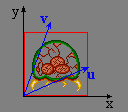
Fig 10.6: Mapping process as seen by computers. u and v (in texture space) are the columns of B and are mapped to the principle axes in screen space.
“Hello, I am Cearn’s GBA. I’m a lean, mean gaming machine that fits in your pocket, and I can push pixels like no one else. Except perhaps my owner’s GeForce 4 Ti4200, the bloody show-off. Anyway, one of the things I do is texture mapping. And not just ordinary texture-mapping, I can do cool stuff like rotation and scaling as well. What I do is fill pixels, all I need to know is for you to tell me where I should get the pixel’s color from. In other words, to fill screen pixel q, I need a matrix B that gives me the proper texel p via p = B · q. I’ll happily use any matrix you give me; I have complete confidence in your ability to supply me with the matrix for the transformation you require.”
Resolution
I hope you spotted the crucial difference between the two points of view. A maps from texture space to screen space, while B does the exact opposite (i.e., ). I think you know which one you should give the GBA by now. That’s right: P = B, not A. This one bit of information is the crucial piece of the affine matrix puzzle.
So now you can figure out P’s elements in two ways. You can stick to the human POV and invert the matrix at the end. That’s why I gave you the inverses of the affine transformations as well. You could also try to see things in the GBA’s way and get the right matrix directly. Tonc’s main affine functions (tonc_video.h, tonc_obj_affine.c and tonc_bg_affine.c) do things the GBA way, setting P directly; but inverted functions are also available using an “_inv” affix. Mind you, these are a little slower. Except for when scaling is involved; then it’s a lot slower.
In case you’re curious, the proper matrix for scale by (, ) and counter-clockwise rotation by α is:
Using the inverse matrices given earlier, we find
The affine matrix P maps from screen space to texture space, not the other way around!
In other words:
: texture x-increment / pixel
: texture x-increment / scanline
: texture y-increment / pixel
: texture y-increment / scanline
Finishing up
Knowing what the P-matrix is used for is one thing, knowing how to use them properly is another. There are three additional points you need to remember when you’re going to deal with affine objects/backgrounds and the affine matrices.
- Datatypes
- Luts
- Initialisation
Data types of affine elements
Affine transformations are part of mathematics and, generally speaking, math numbers will be real numbers. That is to say, floating point numbers. However, if you were to use floating points for the P elements, you’d be in for two rude surprises.
The first one is that the matrix elements are not floats, but integers. The reason behind this is that the GBA has no floating point unit! All floating-point operations have to be done in software and without an FPU, that’s going to be pretty slow. Much slower than integer math, at any rate. Now, when you think about this, it does create some problems with precision and all that. For example, the (co)sine and functions have a range between −1 and 1, a range which isn’t exactly large when it comes to integers. However, the range would be much greater if one didn’t count in units of 1, but in fractions, say in units of 1/256. The [−1, +1] range then becomes [−256, +256],
This strategy of representing real numbers with scaled integers is known as fixed point arithmetic, which you can read more about in this appendix and on wikipedia. The GBA makes use of fixed point for its affine parameters, but you can use it for other things as well. The P-matrix elements are 8.8 fixed point numbers, meaning a halfword with 8 integer bits and 8 fractional bits. To set a matrix to identity (1s on the diagonals, 0s elsewhere), you wouldn’t use this:
    // Floating point == Bad!!
    pa= pd= 1.0;
    pb= pc= 0.0;
but this:
    // .8 Fixed-point == Good
    pa= pd= 1<<8;
    pb= pc= 0;
In a fixed point system with Q fractional bits, ‘1’ (‘one’) is represented by or 1<<Q, because simply that’s how fractions work.
Now, fixed point numbers are still just integers, but there are different types of integers, and it is important to use the right ones. 8.8f are 16bit variables, so the logical choice there is short. However, this should be a signed short: s16, not u16. Sometimes is doesn’t matter, but if you want to do any arithmetic with them they’d better be signed. Remember that internally the CPU works in words, which are 32bit, and the 16bit variable will be converted to that. You really want, say, a 16bit “−1” (0xFFFF) to turn into a 32bit “−1” (0xFFFFFFFF), and not “65535” (0x0000FFFF), which is what happens if you use unsigned shorts. Also, when doing fixed point math, it is recommended to use signed ints (the 32bit kind) for them, anything else will slow you down and you might get overflow problems as well.
Use 32-bit signed ints for affine temporaries
Of course you should use 32bit variables for everything anyway (unless you actually want your code to bloat and slow down). If you use 16bit variables (short or s16), not only will your code be slower because of all the extra instructions that are added to keep the variables 16bit, but overflow problems can occur much sooner.
Only in the final step to hardware should you go to 8.8 format. Before that, use the larger types for both speed and accuracy.
LUTs
So fixed point math is used because floating point math is just to slow for efficient use. That’s all fine and good for your own math, but what about mathematical functions like sin() and cos()? Those are still floating point internally (even worse, doubles!), so those are going to be ridiculously slow.
Rather than using the functions directly, we’ll use a time-honored tradition to weasel our way out of using costly math functions: we’re going to build a look-up table (LUT) containing the sine and cosine values. There are a number of ways to do this. If you want an easy strategy, you can just declare two arrays of 360 8.8f numbers and fill them at initialization of your program. However, this is a poor way of doing things, for reasons explained in the section on LUTs in the appendix.
Tonclib has a single sine lut which can be used for both sine and cosine values. The lut is called sin_lut, a const short array of 512 4.12f entries (12 fractional bits), created by my excellut lut creator. In tonc_math.h you can find two inline functions that retrieve sine and cosine values:
//! Look-up a sine and cosine values
/*! \param theta Angle in [0,FFFFh] range
*   \return .12f sine value
*/

INLINE s32 lu_sin(uint theta)
{   return sin_lut[(theta>>7)&0x1FF];           }

INLINE s32 lu_cos(uint theta)
{   return sin_lut[((theta>>7)+128)&0x1FF];     }
Now, note the angle range: 0-10000h. Remember you don’t have to use 360 degrees for a circle; in fact, on computers it’s better to divide the circle in a power of two instead. In this case, the angle is in 216 parts for compatibility with BIOS functions, which is brought down to a 512 range inside the look-up functions.
Initialization
When flagging a background or object as affine, you must enter at least some values into pa-pd. Remember that these are zeroed out by default. A zero-offset means it’ll use the first pixel for the whole thing. If you get a single-colored background or sprite, this is probably why. To avoid this, set P to the identity matrix or any other non-zero matrix.
Tonc’s affine functions
Tonclib contains a number of functions for manipulating the affine parameters of objects and backgrounds, as used by the OBJ_AFFINE and BG_AFFINE structs. Because the affine matrix is stored differently in both structs you can’t set them with the same function, but the functionality is the same. In table 10.2 you can find the basic formats and descriptions; just replace foo with obj_aff or bg_aff and FOO with OBJ or BG for objects and backgrounds, respectively. The functions themselves can be found in tonc_obj_affine.c for objects, tonc_bg_affine.c for backgrounds, and inlines for both in tonc_video.h … somewhere.
| Function | Description |
|---|---|
| void foo_copy(FOO_AFFINE *dst, const FOO_AFFINE *src, uint count); | Copy affine parameters |
| void foo_identity(FOO_AFFINE *oaff); | |
| void foo_postmul(FOO_AFFINE *dst, const FOO_AFFINE *src); | Post-multiply: |
| void foo_premul(FOO_AFFINE *dst, const FOO_AFFINE *src); | Pre-multiply: |
| void foo_rotate(FOO_AFFINE *aff, u16 alpha); | Rotate counter-clockwise by α·π/8000h. |
| void foo_rotscale(FOO_AFFINE *aff, FIXED sx, FIXED sy, u16 alpha); | Scale by and , then rotate counter-clockwise by α·π/8000h. |
| void foo_rotscale2(FOO_AFFINE *aff, const AFF_SRC *as); | As foo_rotscale(), but input stored in an AFF_SRC struct. |
| void foo_scale(FOO_AFFINE *aff, FIXED sx, FIXED sy); | Scale by and |
| void foo_set(FOO_AFFINE *aff, FIXED pa, FIXED pb, FIXED pc, FIXED pd); | Set P's elements |
| void foo_shearx(FOO_AFFINE *aff, FIXED hx); | Shear top-side right by |
| void foo_sheary(FOO_AFFINE *aff, FIXED hy); | Shear left-side down by |
Sample rot/scale function
My code for a object version of the scale-then-rotate function (à la eq 10.4) is given below. Note that it is from the computer’s point of view, so that sx and sy scale down. Also, the alpha alpha uses 10000h/circle (i.e., the unit of α is π/8000h = 0.096 mrad, or 180/8000h = 0.0055°) and the sine lut is in .12f format, which is why the shifts by 12 are required. The background version is identical, except in name and type. If this were C++, templates would have been mighty useful here.
void obj_aff_rotscale(OBJ_AFFINE *oaff, int sx, int sy, u16 alpha)
{
    int ss= lu_sin(alpha), cc= lu_cos(alpha);

    oaff->pa= cc*sx>>12;    oaff->pb=-ss*sx>>12;
    oaff->pc= ss*sy>>12;    oaff->pd= cc*sy>>12;
}
With the information in this chapter, you know most of what you need to know about affine matrices, starting with why they should be referred to affine matrices, rather than merely rotation or rot/scale or the other names you might see elsewhere. You should now know what the thing actually does, and how you can set up a matrix for the effects you want. You should also know a little bit about fixed point numbers and luts (for more, look in the appendices) and why they’re Good Things; if it hadn’t been clear before, you should be aware that the choice of the data types you use actually matters, and you should not just use the first thing that comes along.
What has not been discussed here is how you actually set-up objects and backgrounds to use affine transformation, which is what the next two chapters are for. For more on affine transformations, try searching for ‘linear algebra’